Identifying and Processing the Targets
Once an image is captured, the next step is to identify Vision Target(s) in the image. This document will walk through one approach to identifying the 2016 targets. Note that the images used in this section were taken with the camera intentionally set to underexpose the images, producing very dark images with the exception of the lit targets, see the section on Camera Settings for details.
Additional Options
This document walks through the approach used by the example code provided in LabVIEW (for PC or roboRIO), C++ and Java. In addition to these options teams should be aware of the following alternatives that allow for vision processing on the Driver Station PC or an on-board PC:
Original Image
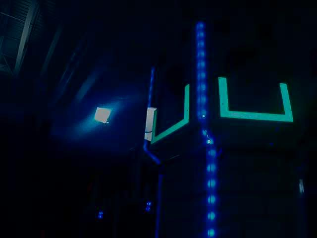
The image shown below is the starting image for the example described here. The image was taken using the green ring light available in FIRST Choice. combined with an additional ring light of a different size. Additional sample images are provided with the vision code examples.
What is HSL/HSV?
The Hue or tone of the color is commonly seen on the artist’s color wheel and contains the colors of the rainbow Red, Orange, Yellow, Green, Blue, Indigo, and Violet. The hue is specified using a radial angle on the wheel, but in imaging the circle typically contains only 256 units, starting with red at zero, cycling through the rainbow, and wrapping back to red at the upper end. Saturation of a color specifies amount of color, or the ratio of the hue color to a shade of gray. Higher ratio means more colorful, less gray. Zero saturation has no hue and is completely gray. Luminance or Value indicates the shade of gray that the hue is blended with. Black is 0 and white is 255.
The example code uses the HSV color space to specify the color of the target. The primary reason is that it readily allows for using the brightness of the targets relative to the rest of the image as a filtering criteria by using the Value (HSV) or Luminance (HSL) component. Another reason to use the HSV color system is that the thresholding operation used in the example runs more efficiently on the roboRIO when done in the HSV color space.
Masking
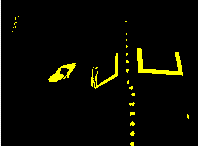
In this initial step, pixel values are compared to constant color or brightness values to create a binary mask shown below in yellow. This single step eliminates most of the pixels that are not part of a target’s retro-reflective tape. Color based masking works well provided the color is relatively saturated, bright, and consistent. Color inequalities are generally more accurate when specified using the HSL (Hue, Saturation, and Luminance) or HSV (Hue, Saturation, and Value) color space than the RGB (Red, Green, and Blue) space. This is especially true when the color range is quite large in one or more dimension.
Notice that in addition to the target, other bright parts of the image (overhead light and tower lighting) are also caught by the masking step.
Notice that in addition to the target, other bright parts of the image (overhead light and tower lighting) are also caught by the masking step.
Particle Analysis
After the masking operation, a particle report operation is used to examine the area, bounding rectangle, and equivalent rectangle for the particles. These are used to compute several scored terms to help pick the shapes that are most rectangular. Each test described below generates a score (0-100) which is then compared to pre-defined score limits to decide if the particle is a target or not.
Coverage Area
The Area score is calculated by comparing the area of the particle compared to the area of the bounding box drawn around the particle. The area of the retroreflective strips is 80 square inches. The area of the rectangle that contains the target is 240 square inches. This means that the ideal ratio between area and bounding box area is 1/3. Area ratios close to 1/3 will produce a score near 100, as the ratio diverges from 1/3 the score will approach 0.
Aspect Ratio
The aspect ratio score is based on (Particle Width / Particle Height). The width and height of the particle are determined using something called the “equivalent rectangle”. The equivalent rectangle is the rectangle with side lengths x and y where 2x+2y equals the particle perimeter and x*y equals the particle area. The equivalent rectangle is used for the aspect ratio calculation as it is less affected by skewing of the rectangle than using the bounding box. When using the bounding box rectangle for aspect ratio, as the rectangle is skewed the height increases and the width decreases.
The target is 20” wide by 12” tall, for a ratio of 1.6. The detected aspect ratio is compared to this ideal ratio. The aspect ratio score is normalized to return 100 when the ratio matches the target ratio and drops linearly as the ratio varies below or above.
Moment
The moment measurement calculates the particles moment of inertia about it’s center of mass. This measurement provides a representation of the pixel distribution in the particle. The ideal score for this test is ~0.28. See: Moment of Inertia
X/Y Profiles
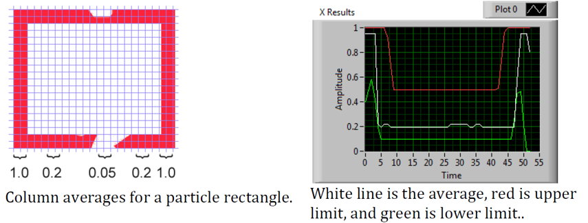
The edge score describes whether the particle matches the appropriate profile in both the X and Y directions. As shown, it is calculated using the row and column averages across the bounding box extracted from the original image and comparing that to a profile mask. The score ranges from 0 to 100 based on the number of values within the row or column averages that are between the upper and lower limit values.
Measurements
If a particle scores well enough to be considered a target, it makes sense to calculate some real-world measurements such as position and distance. The example code includes these basic measurements, so let’s look at the math involved to better understand it.
Position
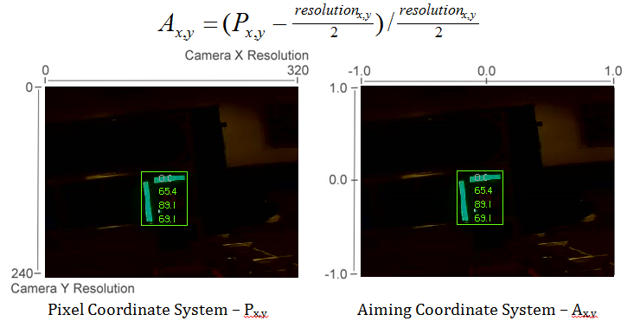
The target position is well described by both the particle and the bounding box, but all coordinates are in pixels with 0,0 being at the top left of the screen and the right and bottom edges determined by the camera resolution. This is a useful system for pixel math, but not nearly as useful for driving a robot; so let’s change it to something that may be more useful.
To convert a point from the pixel system to the aiming system, we can use the formula shown below.
The resulting coordinates are close to what you may want, but the Y axis is inverted. This could be corrected by multiplying the point by [1,-1] (Note: this is not done in the sample code). This coordinate system is useful because it has a centered origin and the scale is similar to joystick outputs and RobotDrive inputs.
Distance
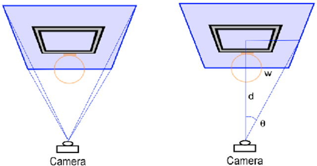
The target distance is computed with knowledge about the target size and the camera optics. The approach uses information about the camera lens view angle and the width of the camera field of view. Shown below-left, a given camera takes in light within the blue pyramid extending from the focal point of the lens. Unless the lens is modified, the view angle is constant and equal to 2Θ. As shown to the right, the values are related through the trigonometric relationship of …
tanΘ = w/d
The datasheets for the cameras can be found at the following URLs: Axis 206, AxisM1011, Axis M1013, Lifecam HD3000. These give rough horizontal view angles for the lenses. Remember that this is for entire field of view, and is therefore 2Θ. This year’s code uses the vertical field-of-view and it is therefore highly recommend to perform calibration (as described in the next article) to determine the appropriate view angle for your camera (empirically determined values for each camera type are included in the code as a reference).
Distance Continued
The next step is to use the information we have about the target to find the width of the field of view the blue rectangle shown above. This is possible because we know the target rectangle size in both pixels and feet, and we know the FOV rectangle width in pixels. We can use the relationships of …
Tft/Tpixel = FOVft/FOVpixel and FOVft = 2*w = 2*d*tanΘ
to create an equation to solve for d, the distance from the target:
d = Tft*FOVpixel/(2*Tpixel*tanΘ)
Notice that the datasheets give approximate view angle information. When testing, it was found that the calculated distance to the target tended to be a bit short. Using a tape measure to measure the distance and treating the angle as the unknown it was found that view angles of 41.7˚ for the 206, 37.4˚ for the M1011, and 49˚ for the M1013 gave better results. Information on performing your own distance calibration is included in the next article.